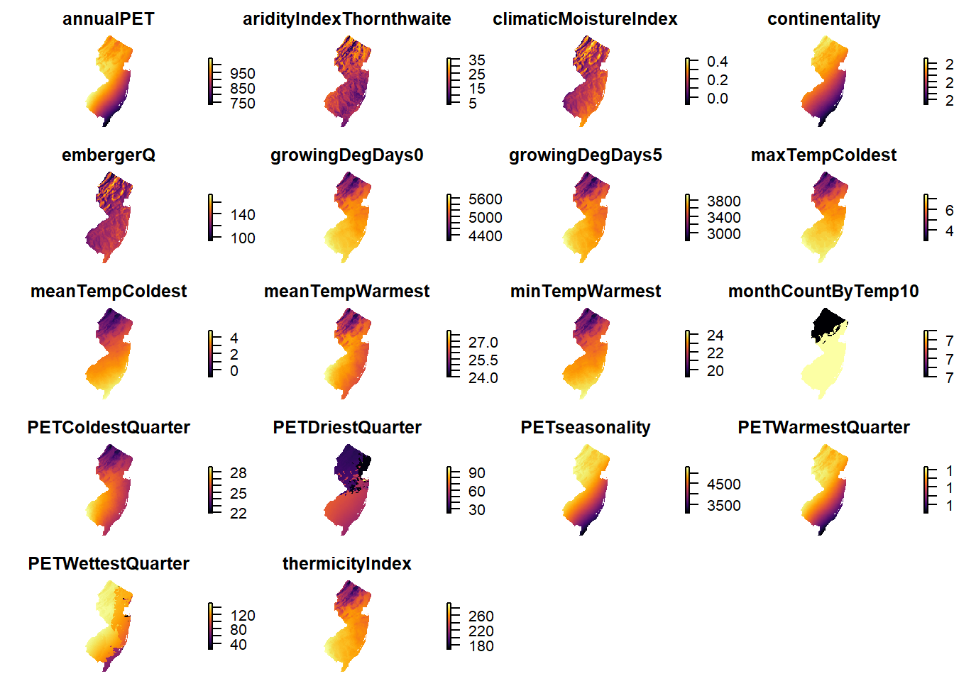
Chapter 4 Co-Variates and Raster Files

4.1 CHELSA global downscaled climate data set

Let me know if you want to see the technical process of modifying raster files using the NJ shapefile.

library(raster)  
library(rgeos)  
library(maps)  
library(viridis)  
library(rgdal)  
library(sf)  

# Example: Reading Raster Files from Source folder to R
```{r setup, include=FALSE}
library(raster)  

# Read in Covariates from Folder name (e.g. chelsa) 
fileDir <- "chelsa"  
files <- list.files(fileDir, pattern = '.tif$', full.names = TRUE)  
```

# Stacked all files
covs <- stack(files)
# Check the names
names(covs)

##  [1] "annualPET"                "aridityIndexThornthwaite"
##  [3] "climaticMoistureIndex"    "continentality"          
##  [5] "embergerQ"                "growingDegDays0"         
##  [7] "growingDegDays5"          "maxTempColdest"          
##  [9] "meanTempColdest"          "meanTempWarmest"         
## [11] "minTempWarmest"           "monthCountByTemp10"      
## [13] "PETColdestQuarter"        "PETDriestQuarter"        
## [15] "PETseasonality"           "PETWarmestQuarter"       
## [17] "PETWettestQuarter"        "thermicityIndex"

# make a Plot of the Covariates

4.2 Covariates plot

par(mfrow = c(5, 4), mar = c(0.5, 0.5, 2, 0))

for (i in 1:nlayers(covs)) {
  plot(covs[[i]], col = inferno(100), box = FALSE, axes = FALSE)
  title(main = names(covs)[i])
}

Examples of Chelsa satellite data used as SOC covariates in this study